Notebook 1: Introduction to Jupyter and Python
Contents
Notebook 1: Introduction to Jupyter and Python #
Before we can begin analyzing protein PDB files, we need to cover some Python and Jupyter notebook basics. This notebook will not make you an expert programmer, but it will give you a quick foundation on skills you will need for the subsequent notebooks. The goals of this notebook are to:
Familiarize everyone with running a Jupyter notebook
Provide some basic Python we will use later in this activity including functions and basic plotting
1. Jupyter Notebooks #
Jupyter notebooks are a shareable and interactive electronic document that contains two main types of cells: code and markdown. The code cells contain live code that can be executed directly inside the Jupyter notebook with any output appearing directly below the code cell. Markdown cells can contain text, equation, and images to provide background and instructions to the user.
To provide rich content in the markdown cells, equations can be formated using Latex-like syntax (example below), and text can be formated using either the lightweight markdown language or html.
Example equation: $\( E = E^o - \frac{RT}{nF}lnQ \)$
4 + 7
11
2. Python Functions #
The following is a (very) quick introduction to using functions in Python as we will be using this skill in this activity. Python allows the use of functions provided natively with every Python installation. If you are interested in learning more, there are additional resouces at the bottom of this notebook. The general structure of a function is below where \(func\) is the function name, and any input is placed inside the parentheses.
For example, abs() is the absolute value function that comes with Python.
abs(-655)
655
Python also includes series of modules containing more functions, and a list of these modules can be found at https://docs.python.org/3/py-modindex.html. Before these modules can be used, they must to be imported, which is how Python loads them into memory. The general format is import <module>.
import math
Once a module has been imported, any function in that module may be executed using the format module.func(). For example, there is a square root function in the math module called sqrt(). To call (i.e., run) this function, we need to type math.sqrt().
math.sqrt(25)
5.0
Function Docstrings#
If you’re not sure how to use and function or what it does, place the cursor in or after the parentheses of the fucntion and press Shift + Tab. The Docstring will appea providing a breif description and/or set of instructions
math.degrees(3.14159)
179.9998479605043
math.pow(2, 3)
8.0
3. External Libraries #
While Python comes with an impressive collection of modules, there are often tasks that users want to complete that are not covered with the native Python modules. For this, users can import external libraries. A list of common Python scientific libraries are listed below with breif description.
Libraries can contain submodules which are collections of functions/data with a similar theme or purpose. Examples of submodules in the SciPy library are listed below as an example.
SciPy: includes common function for scientific data processing tasks like signal processing, interpolation, optimization, etc…
signal: signal processing tools
fft: fast Fourier processing tools
optimize: optimization tools
integrate: integration functions
stats: statistics functions
constants: collection of scientific constants
NumPy: basic library to handeling larger amounts of data and includes additional mathematical functions
Pandas: more advanced library for handeling data
Matplotlib: standard data plotting and visuallization library
Seaborn: more advanced data plotting and visualization library
SymPy: symbolic mathematics library
Biopython: bioinformatics library
Scikit-image: scientific image processing library
Scikit-learn: general purpose machine learning library
Almost all of the above libraries come with the Anaconda installation of Python, so you should have most of these already installed (except Biopython).
4. Plotting with Matplotlib #
Matplotlib is a common plottling library using with Python to visualize data. The following commands need to be run in order to import the matplotlib library and to set plotting to display the outputs inside the Jupyter notebook, respectively.
import matplotlib.pyplot as plt
%matplotlib inline
import matplotlib.pyplot as plt
%matplotlib inline
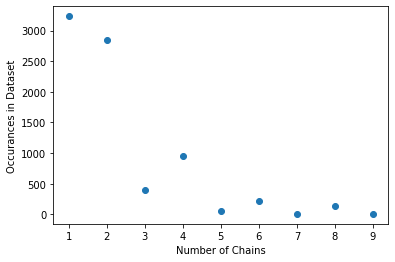
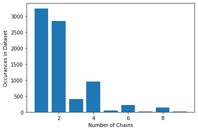
Proteins may be composed of a single peptide chain or multiple peptide chains. Below is some data on the number of structures in the Top8000 dataset that contains 1 \(\rightarrow\) 9 peptide chains.
Note: some structures in the Top8000 dataset contain more peptide chains that nine, but for this activity, we will focus on 1 \(\rightarrow\) 9.
chains = [1,  2,  3,  4,  5,  6,  7,  8,  9]
counts = [3235, 2847, 403, 953, 47, 223, 7, 137, 7]
We can plot data as a scatter plot using the plt.scatter() function. This function requires the x and y data as shown below.
plt.scatter(x, y)
The following lines can also be included to add title, x-labels, and y-labels on the plot. Be sure to keep the quotes around your text!
plt.title('Text')
plt.xlabel('Text')
plt.ylabel('Text')
plt.scatter(chains, counts)

plt.xlabel('Number of Chains')
plt.ylabel('Occurances in Dataset')
Text(0, 0.5, 'Occurances in Dataset')

Matplotlib Functions #
Matplotlib includes a series of functions for generating different types
plt.scatter(x,y): yields scatter plot with just markersplt.plot(x,y): yields line plot, markers optionalplt.bar(x,y): yields bar plotplt.stem(x,y): yields stem plot (like scatter plot with lines to x-axisplt.boxplot(x,y): yields box plotplt.hist(nums): yields histogram plot showing distribution of values in datasetplt.pie(nums): yields a pie plot showing relative ratios
plt.bar(chains, counts)

plt.xlabel('Number of Chains')
plt.ylabel('Occurances in Dataset')
Text(0, 0.5, 'Occurances in Dataset')

Plotting Activity#
Below is a series of data either included in the Jupyter notebook or imported from an external file. Follow the instructions to visualize these data.
a. Other Plotting Types #
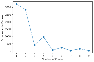
Display the above oligomer data using the following plotting function.
plt.plot(x, y, 'o--')
The o- tells the function to use circles for markers and to connect them with a line. Other markers (e.g.,p, ^, or s) or line types (e.g., -- or -.) can be used if desired.
plt.plot(chains, counts, 'o--')

plt.xlabel('Number of Chains')
plt.ylabel('Occurances in Dataset')
Text(0, 0.5, 'Occurances in Dataset')

b. Hisogram Plots#
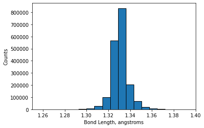
A histogram plot is a frequency plot that shows how many values fall within each set of ranges known as bins. It looks like a bar plot except that the width of the bars is significant and the histogram function automatically tallies the data to see how many values go in each bin. The matplotlib histogram function is shown below. The first example only provides the data and allows the function to choose how many bins are appropriate. The second example provides the plotting function both the data and explicitly mandates that the data be sorted into 10 bins. You can change the number of bins to suit your data.
plt.hist(data)

plt.hist(data, bins=10)
If you want to zoom in on the graph, you can set the x-axis limits using the plt.xlim() function. Just add it to another line in the same code cell as the main plotting function.
plt.xlim(min, max)
Below is code that loads peptide bond length data from an external file into the variable lengths. Visualize these data using a histogram plot.
import numpy as np
lengths = np.genfromtxt('amide_bond_lengths.csv', delimiter=',')
plt.hist(lengths, bins=200, edgecolor='k')
plt.xlabel('Bond Length, angstroms')
plt.xlim(1.25, 1.4)
plt.ylabel('Counts')
plt.show()

Additional Resources #
Additional resources for learning Python and plotting are listed below.
Scientific Computing for Chemists is a free electronic textbook for learning and teaching Python, Jupyter notebooks, and applying these skills to solving chemical problems available at https://github.com/weisscharlesj/SciCompforChemists
The offical Python website is a good resource about pure Python
For information about SciPy and the SciPy stack, see the SciPy Website

