Chapter 2: Intermediate Python

The contents of this chapter are intended for those who wish to dive deeper into the Python programming language. Many of the topics herein are not strictly required for most subsequent chapters but will make you more efficient and effective as a Python programmer. Items from this chapter are occasionally used in subsequent chapters, but you should still be able to follow along without having read this chapter. If you are in a rush, you can bypass this chapter and circle back as needed. The sections and sometimes subsections of this chapter may also be read in any order or as needed.

2.1 Syntactic Sugar

Syntactic sugar is a nickname given to any part of a programming language that does not extend the capabilities of the language. If any of these features were suddenly removed from the language, the language would still be just as capable, but the advantage of anything labeled “syntactic sugar” is that it makes the code quicker/shorter to write or easier to read. Below are a few examples from the Python language that you are likely to come across and find useful.

2.1.1 Augmented Assignment

Augmented assignment is a simple example of syntactic sugar that allows the user to modify the value assigned to a variable. If we want to increase a value by one, we can recursively assign the variable to itself plus one as shown below.

x = 5

x = x + 1 
x

6

This is certainly not difficult, but it does involve typing the variable more than once which becomes less desirable as your variable names get longer. As an alternative, we can also use augmented assignment shown below that accomplishes the same task. The += means “increment.”

x += 1
x

7

Augmented assignment can also be used with addition, subtraction, multiplication, and division as shown in Table 1.

Table 1 Augmented Assignment

Augmented Assignment	Regular Assignment	Description
x += a	x = x + a	Increments the value
x -= a	x = x - a	Decrements the value
x *= a	x = x * a	Multiplies the value
x /= a	x = x / a	Divides the value

2.1.2 List Comprehension

At this point, you may have noticed that it is fairly common to generate a list populated with a series of numbers. If the values are evenly spaced integers, simply use the range() function and covert it to a list using list(). In all other scenarios, you will need to create an empty list, use a for loop to calculate the values, and append the values to the list as they are generated. Below is an example of generating a list of squares of all integers from 0 \(\rightarrow\) 9 using this method.

squares = []
for integer in range(10):
    sqr = integer**2
    squares.append(sqr)

squares

[0, 1, 4, 9, 16, 25, 36, 49, 64, 81]

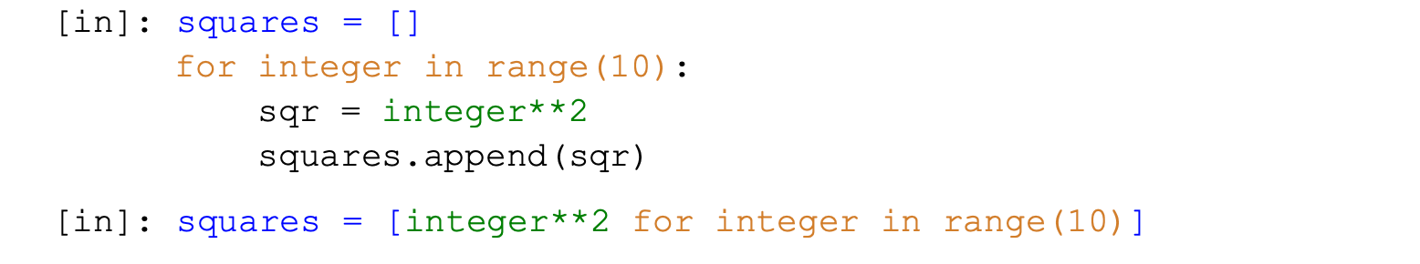
This whole process can be compressed down into a single line by expressing the for loop in square brackets resulting in the following. This is known as list comprehension.

Note

Python also supports analogous code structures for creating other objects such as tuple comprehension and dictionary comprehension which will not be covered here.

squares = [integer**2 for integer in range(10)]
squares

[0, 1, 4, 9, 16, 25, 36, 49, 64, 81]

To help you visualize where each part comes from, below are both methods again but with common sections in the same colors.

List comprehension can take a little time to get used to, but it is well worth it. It saves both time and space and makes the code less cluttered.

Note

In addition to list comprehension, there are the related dictionary comprehension and set comprehension shown below that can be used for dictionary and set objects introduced in the following two sections.

[1]: {n: 2*n**2 for n in range(5)}
[1]: {0: 0, 1: 2, 2: 8, 3: 18, 4: 32, 5: 50}

[2]: {(n, 2*n**2) for n in range(5)}
[2]: {(0, 0), (1, 2), (2, 8), (3, 18), (4, 32)}

2.1.3 Compound Assignment

At the beginning of a program or calculations, it is often necessary to populate a series of variables with values. Each variable may get its own line in the code, and if there are numerous variables, this can clutter your code. An alternative is to assign multiple variables in the same assignment as shown below with atomic masses of the first three elements.

H, He, Li = 1.01, 4.00, 5.39

H

1.01

Each variable is assigned to the respective value. This is known as tuple unpacking as H, He, Li and 1.01, 4.00, 5.39 are automatically turned into tuples by Python (behind the scenes) as demonstrated below.

1.01, 4.00, 5.39

(1.01, 4.0, 5.39)

Therefore, the above assignments are an equivalent of the following code.

(H, He, Li) = (1.01, 4.00, 5.39)

2.1.4 Lambda Functions

The lambda function is an anonymous function for generating simple Python functions. Their value is that they can be used to generate functions in fewer lines of code than the standard def statement, and they do not necessarily need to be assigned to a variable… hence the anonymous part. The latter is useful in applications that require a Python function but the user does not want to clutter the namespace by assigning it to a variable or take the time to define a function normally. The lambda function is defined as shown below with the variable immediately after the lambda statement as the independent variable in the function.

lambda x: x**2

<function __main__.<lambda>(x)>

Being that it is not attached to a variable, it needs to be used immediately. Alternatively, it can be attached to a variable as shown below and then operates like any other Python function.

f = lambda x: x**2

f(9)

81

As an example looking ahead to chapter 8, the quad() function from the scipy.integrate module is a general-purpose method for integrating the area under mathematical functions. Along with the upper and lower limits, the integration functions require a mathematical function in the form of a Python function (i.e., not just a mathematical expression). This would ordinarily require a formally-defined Python function, but it is often more convenient to use a lambda function as a single use Python function as shown below. In the following example, we use integration to find the probability of finding a particle in the lowest state between 0 and 0.4 in a box of length 1 by performing the following integration.

\[ p = 2 \int_0^{0.4} sin^2(\pi x) \]

from scipy.integrate import quad
import math

quad(lambda x: 2 * math.sin(math.pi*x)**2, 0, 0.4)

(0.30645107162113616, 3.402290356348383e-15)

def particle_box(x):
    return 2 * math.sin(math.pi*x)**2

quad(particle_box, 0, 0.4)

(0.30645107162113616, 3.402290356348383e-15)

The first value in the returned tuple is the result of the integration, and the second value is the estimated uncertainty. Therefore, the particle has about a 30.6% probability of being found in the region of 0 \(\rightarrow\) 0.4. Performing this same calculation by defining the function with def is shown below. This requires more lines of code than a lambda expression.

2.2 Dictionaries

Python dictionaries are a multi-element Python object type that connects keys and values analogous to the way a real dictionary connects a word (the key) with a definition (the value). These are also known as associative arrays. Dictionaries allow the user to access the stored values using a key without knowing anything about order of items in the dictionary. One way to think of a dictionary is an object full of variables and assigned values. For example, if we are looking to write a scrip to calculate the molecular weight of a compound based on its molecular formula, we would need access to the atomic mass of each element based on the elemental symbol. Here the key is the symbol and the value is the atomic mass. It looks something like a list with curly brackets and each item is a key:value pair separated by a colon. Below is an example of a dictionary containing the atomic masses of the first ten elements on the periodic table.

AM = {'H':1.01, 'He':4.00, 'Li':6.94, 'Be':9.01,
      'B':10.81, 'C':12.01, 'N':14.01, 'O':16.00,
      'F':19.00, 'Ne':20.18}

With the dictionary in hand, we can access the mass of any element in it using the atomic symbol as the key.

AM['Li']

6.94

Even though it is traditional to call them key:value pairs, the value does not need to be a numerical value. It can also be a string or other object type, and the key can also be any object type.

If you ever find yourself with a dictionary and not knowing the keys, you can find out using the keys() dictionary method.

AM.keys()

dict_keys(['H', 'He', 'Li', 'Be', 'B', 'C', 'N', 'O', 'F', 'Ne'])

We can also get a look at the key:value pairs using the items() method or iterate over the dictionary to get access to keys, values, or both.

AM.items()

dict_items([('H', 1.01), ('He', 4.0), ('Li', 6.94), ('Be', 9.01), ('B', 10.81), ('C', 12.01), ('N', 14.01), ('O', 16.0), ('F', 19.0), ('Ne', 20.18)])

for key, values in AM.items():
    print(values)

1.01
4.0
6.94
9.01
10.81
12.01
14.01
16.0
19.0
20.18

Additional key:value pairs can be added to an already existing dictionary by calling the key and assigning it to a value as demonstrated below. Instead of giving an error, the dictionary inserts that key: value pair.

AM['Na'] = 22.99
AM

{'H': 1.01,
 'He': 4.0,
 'Li': 6.94,
 'Be': 9.01,
 'B': 10.81,
 'C': 12.01,
 'N': 14.01,
 'O': 16.0,
 'F': 19.0,
 'Ne': 20.18,
 'Na': 22.99}

Notice that after adding sodium to the atomic mass dictionary, the order of all the pairs changed. Unlike a tuple or list, the order in a dictionary does not matter, so it is not preserved.

Another method for generating a dictionary is the dict() function which takes in pair for nested lists or tuples and generates key:value pairs as follows.

dict([('H',1), ('He',2), ('Li',3)])

{'H': 1, 'He': 2, 'Li': 3}

Not only can dictionaries be used to store data used in calculations, such as atomic masses, they can also be used to store changing data as we perform calculations or operations. For example, let’s say we want to count how often each base (i.e., A, T, C, and G) appears in the following DNA sequence DNA. For this, we create a dictionary dna_bases to hold the totals for each base and add one to each value as we iterate along the DNA sequence.

DNA = 'GGGCTCCATTGTCTGCCCGGGCCGGGTGTAGTCTAAGGTT'

dna_bases = {'A':0, 'T':0, 'C':0, 'G':0}
for base in DNA:
    dna_bases[base] += 1

dna_bases

{'A': 4, 'T': 11, 'C': 10, 'G': 15}

2.3 Set

Sets are another Python object type you may encounter and use on occasions. These are multi-element objects similar to lists with the key difference that each element can appear only once in the set. This may be useful in applications where code is taking stock of what is present. For example, if we are taking inventory of the chemical stockroom to know which chemical compounds are on hand for experiments, the names of the compounds can be stored in a set. If more than one bottle of a compound is present in the stockroom, the set only contains the name once because we are only concerned with what is available, not how many are available. A set looks like a list except curly brackets are used instead of square brackets.

compounds = {'ethanol', 'sodium chloride', 'water',
             'toluene', 'acetone'}

We can add additional items to the set using the add() set method.

Note

The method is called add() and not append() as is used for lists because unlike lists, sets do not preserve the order of items contained within them.

compounds.add('calcium chloride')
compounds

{'acetone',
 'calcium chloride',
 'ethanol',
 'sodium chloride',
 'toluene',
 'water'}

compounds.add('ethanol')
compounds

{'acetone',
 'calcium chloride',
 'ethanol',
 'sodium chloride',
 'toluene',
 'water'}

Notice that when ethanol is added to the set, nothing changes. This is because ethanol is already in the set, and sets do not store redundant copies of elements.

Multiple sets can be concatenated or subtracted from each other using the | and – operators, and two sets can be compared using Boolean operators. Below are two sets containing the atomic orbitals in nitrogen (N) and calcium (Ca) atoms. Even though there are three 2p orbitals in nitrogen, it only appears once telling us what types of orbitals are present but not how many.

N = {'1s','2s','2p'}
Ca = {'1s','2s','2p', '3s', '3p', '4s'}

N | Ca # returns orbitals in either set

{'1s', '2p', '2s', '3p', '3s', '4s'}

Ca - N  # returns Ca orbitals minus those in common

{'3p', '3s', '4s'}

N & Ca  # returns orbitals in both sets

{'1s', '2p', '2s'}

Table 2 Python Set Operators

Operator	Name	Description
&	Intersection	Returns items in both sets
-	Difference	Returns items in the first set minus common items in both sets
|	Union	Merges both sets; redundancies are removed automatically
^	Symmetric Difference	Merges both sets minus items in common (i.e., “exclusive or”)

2.4 Python Modules

Remember from the last chapter that a module is a collection of functions and data with a common theme. You have already seen the math module in section 1.1.3, but Python also contains a number of other native modules that come with every installation of Python. Table 3 lists a few common examples, but there are certainly many others worth exploring. You are encouraged to visit the Python website and explore other modules. This section will introduce a few useful modules with some examples of their uses.

Note

See https://docs.python.org/3/py-modindex.html for a more complete listing and descriptions of built-in Python modules.

Table 3 Some Useful Python Modules

Name	Description
os	Provides access to your computer file system
itertools	Iterator and combinatorics tools
random	Functions for pseudorandom number generation
datetime	Handling of date and time information
csv	For writing and reading CSV files
pickle	Preserves Python objects on the file system
timeit	Times the execution of code
audioop	Tools for reading and working with audio files
statistics	Statistics functions

2.4.1 os Module

The os module provides access to the files and directories (i.e., folders) on your computer. Up to this point, we have been opening files that are in the same directory as the Jupyter notebook, so Jupyter has no difficulty finding the files. However, if you ever want to open a file somewhere else on your computer or open multiple files, this module is particularly useful. Below you will learn to use the os module to open files in non-local directories (i.e., not the directory your Jupyter notebook is in) and to open an entire folder of files.

Table 4 Select os Module Functions

Function	Description
os.chdir()	Changes the current working directory to the path provide
os.getcwd()	Returns the current working directory path
os.listdir()	Returns a list of all files in the current or indicated directory

Table 4 provides a description of the three functions that we will be using. To open a file not in the directory of your Jupyter notebook, you will need to change the directory Python is currently looking in, known as the current working directory, using the chdir() method. It takes a single string argument of the path in string format to the folder containing the files of interest. For example, if the files are in a folder called “my_folder” on your computer desktop, you might use something like the following. The exact format will vary depending upon your computer and if you are using macOS, Windows, or Linux.

import os
os.chdir('/Users/me/Desktop/my_folder')

If you are not sure which directory is the current working directory, you can use the getcwd() function. It does not require any arguments.

os.getcwd()

Another useful function from the os module is the listdir() method which lists all the files and directories in a folder. It is useful not only for determining the contents a folder but also for iterating through all the files in a folder. Imagine you have not just a single CSV file with data but an entire folder of similar CSV files that you need to import into Python. Instead of handling these files one at a time, you can have Python iterate through the folder and import each CSV file it finds. Below is a demonstration of importing and printing every CSV file on the computer desktop.

import numpy as np
os.chdir('/Users/me/Desktop') # changes directory
for file in os.listdir():
    if file.endswith('csv'): # only open csv files
        data = np.genfromtxt(file)
        print(data)

The code above goes through every file on the computer desktop, and if the file name ends in “csv”, Python imports and prints the contents. Checking the file extension is an important step even if you have a folder that you believe only contains CSV files. This is because folders on many computers contain invisible files for use by the computer operating system. The user usually cannot see them, but Python can and will generate an error if it tries to open it as a CSV file. Checking the file extension ensures that Python only tries to open the CSV files.

2.4.2 itertools Module

The itertools modules contains an assortment of tools for looping over data in an efficient manner. There are a number of functions that are good to know from this module, but we will focus on the combinatorics functions combinations() and permutations().

The combinations(collection, n) function generates all n-sized combinations of elements from a collection such as a list, tuple, or range object. With combinations(), order does not matter, so (1, 2) is equivalent to (2, 1). In the below code, the combinations() functions generates all pairs of elements from numbers.

import itertools
numbers = range(5)

itertools.combinations(numbers, 2)

<itertools.combinations at 0x1048f9710>

So what just happened? Instead of returning a list, it returned a combinations object. You do not need to know much about these except that they can be converted into lists or iterated over to extract their elements, and they are single use. Once you have iterated over them, they need to be generated again if you need them again.

Note

combinations() is a type of function called a generator. It only generates values on demand in an effort to reduce the memory usage. This is similar to the range() function.

for pair in itertools.combinations(numbers, 2):
    print(pair)

(0, 1)
(0, 2)
(0, 3)
(0, 4)
(1, 2)
(1, 3)
(1, 4)
(2, 3)
(2, 4)
(3, 4)

Each combination is returned in a tuple, and if the combination object is converted to a list, it would be a list of tuples.

The permutations() function is very similar to combinations(), except with permutations(), order matters. Therefore, (2, 1) and (1, 2) are inequivalent. This is especially important in probability and statistics. Permutations of a group of items can be generated just like in the combinations examples above.

for pair in itertools.permutations(numbers, 2):
    print(pair)

(0, 1)
(0, 2)
(0, 3)
(0, 4)
(1, 0)
(1, 2)
(1, 3)
(1, 4)
(2, 0)
(2, 1)
(2, 3)
(2, 4)
(3, 0)
(3, 1)
(3, 2)
(3, 4)
(4, 0)
(4, 1)
(4, 2)
(4, 3)

Notice how (0, 2) and (2, 0) are both present in the permutations while only one is listed in the combinations.

2.4.3 random Module

The random module provides a selection of functions for generating random values. Random values can be integers or floats and can be generated from a variety of ranges and distributions. A selection of common functions from the random module are shown in Table 5. We will not go into much detail here as random value generation is covered in significantly more detail at the end of chapter 4. One key limitation of the random module is that the functions typically only generate a single value at a time. If you want multiple random values, you need to either use a loop or use the random value functions from NumPy presented in chapter 4.

Table 5 Functions from random Module

Function	Description
random.random()	Generates a value from [0, 1)
random.uniform(x, y)	Generates a float from the range [x, y) with a uniform probability
random.randrange(x, y)	Generates an integer from the provided range [x, y)
random.choice()	Randomly selects an item from a list, tuple, or other multi-element object
random.shuffle()	Shuffles a multi-element object

One point worth noting is that square brackets mean inclusive while the parentheses mean exclusive, so [0, 9) means from 0 \(\rightarrow\) 9 including 0 but not including 9.

import random
random.random()

0.7525034831980151

random.randrange(0, 10)

4

a = [1,2,3,4,5,6]
random.shuffle(a)
a

[3, 4, 1, 5, 2, 6]

2.5 Zipping and Enumeration

There are times when it is neccesary to iterate over two lists simultaneously. For example, let us say we have a list of the atomic numbers (AN) and a list of approximate atomic masses (mass) of the most abundant isotopes for the first six elements on the periodic table.

AN = [1, 2, 3, 4, 5, 6]
mass = [1, 4, 7, 9, 11, 12]

If we want to calculate the number of neutrons in each isotope, we need to subtract each atomic number (equal to the number of protons) from the atomic mass. To accomplish this, it would be helpful to iterate over both lists simultaneously. Below are a couple methods of doing this.

2.5.1 Zipping

The simplest way to iterate over two lists simultaneously is to combine both lists into a single, iterable object and iterate over it once. The zip() function does exactly this by merging two lists or tuples, like a zipper on a jacket, into something like a nested list of lists. However, instead of returning a list or tuple, the zip() function returns a single-use zip object.

zipped = zip(AN, mass)

for pair in zipped:
    print(pair[1] - pair[0])

0
2
4
5
6
6

As noted above, these are single-use objects, so if we try to use it again, nothing happens.

for pair in zipped:
    print(pair[1] - pair[0])

If the two lists are of different length, zip() stops at the end of the shorter list and returns a zip object with a length of the shorter list.

2.5.2 Enumeration

A close relative to zip() is the enumerate() function. Instead of zipping two lists or tuples together, it zips a list or tuple to the index values for that list. Similar to zip(), it returns a one-time use iterable object.

enum = enumerate(mass)

for pair in enum:
    print(pair)

(0, 1)
(1, 4)
(2, 7)
(3, 9)
(4, 11)
(5, 12)

The zip() function can be made to do the same thing by zipping a list with a range object of the same length as shown below, but enumerate() may be slightly more convenient.

zipped = zip(range(len(mass)), mass)
for item in zipped:
    print(item)

(0, 1)
(1, 4)
(2, 7)
(3, 9)
(4, 11)
(5, 12)

2.6 Encoding Numbers

During most of your work in Python, you do not need to think about how and where the values are stored as Python handles this for you. If you assign a number to a variable, Python will determine how to properly store this information. However, there are instances where you will need to understand a little about how numbers are encoded such as in gray scale images (chapter 7).

Numbers on your computer are stored in binary which is a base two numbering system. That is, instead of using digits from 0 \(\rightarrow\) 9 to describe a number, only 0 and 1 are used.

Note

Standard numbers used by humans are a base-ten because we describe values using combinations of ten digits (0, 1, 2, 3, 4, 5, 6, 7, 8, and 9). Once we get to 9, the digit returns to 0 and a 1 is placed to the left. In a binary numbering system, we use only 0 and 1 to describe values. Analogously, once we get to 1, the digit returns to 0 and a 1 is placed to the left. Therefore, “10” is two in binary.

When a number is stored in memory, a fixed block of zeros/ones are allocated to storing this information, and depending upon the size or precision of the number to be stored, this block may need to be larger or smaller. By convention, the blocks are typically 8, 16, 32, 64, or 128 bits (i.e., zeros or ones) in size. Table 6 lists a few examples with the terms used by Python.

Table 6 Python Data Types

Data Type	Description
uint8	Integers from 0 \(\rightarrow\) 255
uint16	Integers from 0 \(\rightarrow\) 65535
uint32	Integers from 0 \(\rightarrow\) 4294967295
int8	Integers from -128 \(\rightarrow\) 127
int16	Integers from -32768 \(\rightarrow\) 32767
int32	Integers from -2147483648 \(\rightarrow\) 2147483647
float32	Singe-precision floating-point numbers
float64	Double-precision floating-point numbers

Probably the simplest way to encode a number is an unsigned 8-bit integer. The “unsigned” means that is cannot have a negative sign while the “8-bit” means it can use eight zeros and ones to describe the number. For example, if we want to encode the number 3, it is 00000011. Even if not all the bits are strictly required, they have been allotted for the storage of this value, and with 8 bits, we can encode numbers from 0 \(\rightarrow\) 255 (i.e., 00000000 \(\rightarrow\) 11111111). If we want to encode any larger numbers, a longer block of bits such as 16 or 32 will need to be allotted.

To encode a negative integers, signed integers are required. The key difference between a signed and unsigned integer is that unsigned are always positive while signed can describe positive and negative values by using the first bit to describe the sign. The first bit is 0 for a positive and 1 for a negative number. Because the first bit is reserved for sign, a signed integer can describe values of only half the magnitude as an unsigned integer of the same bit length. For example, an 8-bit signed integer can describe values from -128 \(\rightarrow\) 127. All combinations of zeros/ones that start with a 0 define positive values from 0 \(\rightarrow\) 127 while all combinations of zeros/ones that start with a 1 define values from -128 \(\rightarrow\) -1. That is, 10000000 equals -128 while 11111111 describes -1.

For non-integer values, we need floats. The number of bits used to describe a float dictates the precision of the value… or rather is the number of decimal places the float extends. The various types listed above support both positive and negative values, and the more bits, the more precision they offer.

2.7 Advanced Functions

Section 1.9 describes positional arguments and keyword arguments as two methods for providing functions with information and instructions, but thus far, these methods have only allowed the function to take a predetermined numbers of arguments. While some flexibility is offered by the ability to set default keyword arguments that users have the option of overriding or leaving as the default, there is still a limit on the number of parameters in the function. What do we do when we need to write a function that takes an unspecified number of arguments? This section provides two approaches to solving this problem.

2.7.1 Variable Positional Arguments

As a possible use case, it is common practice in lab to purify a solid compound by recrystallization, and chemists will often harvest multiple crops of crystals from the same solution to get the highest possible yield. If we want to write a function that returns the percent yield of a synthesized compound using the theoretical yield and the yields of each recrystallization crop, we are faced with the challenge of not knowing how many crops to expect. One solution is a var-positional argument.

The var-positional argument (often *arg), is a positional argument that accepts variable numbers of inputs. The arguments are then stored as a local tuple in the function attached to the arg variable. Even though it is extremely common in examples to see people use arg as the variable, you may use any non-reserved variable you like as long as you precede it with an asterisk in the function definition. For example, a function for calculating the percent yield is shown below with g_theor as the theoretical yield in grams and g_crops as the var-positional parameter storing the mass of each crop of crystals in grams.

def per_yield(g_theor, *g_crops):
    g_total = sum(g_crops)
    percent_yield = 100 * (g_total / g_theor)
    return percent_yield

per_yield(1.32, 0.50, 0.11, 0.27)

66.66666666666666

Interestingly, depending upon how you write the internals of the function, the var-positional argument is not strictly necessary for the function to work. In this case, because sum() function returns 0 if no arguments are passed to it, the per_yield() function still works with no error returned.

per_yield(1.32)

0.0

2.7.2 Variable Keyword Arguments

Similarly, an unspecified number of keyword arguments can also be accepted by a Python function using var-keyword arguments. In this case, the user not only dictates the number of arguments but also picks the variable names. The user-defined variables and values are stored in a local dictionary as key:value pairs. As an example, we can write a function that calculates the molar mass of a compounds based on the number and type of elements it contains. It is certainly possible to write a function with every chemical element as a keyword argument, but this gets absurd with so many chemical elements to choose from. Instead, we can use a var-keyword parameter as demonstrated below. The var-keyword argument is indicated with a ** before the variable name. The function below is only designed to work with the first nine elements for brevity.

def mol_mass(**elements):
    m = {'H':1.008, 'He':4.003, 'Li':6.94, 'Be':9.012,
         'B':10.81, 'C':12.011, 'N':14.007, 'O':15.999,
         'F':18.998}
    masses = []  # mass total from each element
    for key in elements.keys():
        masses.append(elements[key] * m[key])
    return sum(masses)

Let us test this function by calculating the molar mass of caffeine which has a molecular formula of C\(_8\)H\(_{10}\)N\(_4\)O\(_2\).

mol_mass(C=8, H=10, N=4, O=2)

194.194

The user experience would be the same if we wrote the function to accept keyword arguments with default values of zero, but it is sometimes more convenient for the person writing the code to design the function to accept var-keyword arguments.

2.7.3 Recursive Functions

Functions can call other functions. This is probably not surprising as we have already seen functions call math.sqrt() and append(), but what may be surprising is that Python allows a function to call itself. This is known as a recursive function.

If we want to write a function that calculates the remaining mass of radioactive materials after a given number of half-lives, this can be accomplished using a for or while loop, but it can also be accomplished recursively. We start by having the function divide the provided mass (mass) in half and then decrement the number of half-lives (hl) by one. This is the core component of the function. If hl is zero, the function is done and returns the mass. If not, the function calls itself again with the remaining mass and number of half-lives. This is the recursive part. The second time the function is run, the mass is again halved and the half-lives decremented by one, and the number of half-lives is again checked.

def half_life(mass, hl=1):
    '''(float, hl=int) -> float 
    Takes in mass and number of half-lives and returns 
    remaining mass of material. Half-lives need to be 
    integer values.
    '''
    mass /= 2
    hl -= 1
      
    if hl == 0:
        return mass
    else:
        return half_life(mass, hl=hl)

half_life(4.00, hl=2)

1.0

half_life(4.00, hl=4)

0.25

It works! In the second example above, the half_life() function is run four times because the function called itself an additional three times. What happens if we feed the function 1.5 half-lives? Like a while loop with a faulty termination condition, this function will keep going because hl never equals zero. Luckily, Python has a safeguard that stops recursive functions from running more than a thousand iterations, but this is still a problem. We can protect against this issue by doing a check at the start of the function to ensure an integer is provided using the isinstance() function which takes two arguments, the variable and the object type.

isinstance(x, type)

Tip

If you cannot guarantee that the inputs for your code will conform to certain requirements (e.g., be an integer), it is wise to do checks at the start of your code. This is especially true if the input or data for your code comes from people other than the author of the code.

def half_life(mass, hl=1):
    '''(float, hl=int) -> float
    Takes in mass and number of half-lives and returns
    remaining mass of material. Half-lives need to be
    integer values.
    '''

    if not isinstance(hl, int):
        print('Invalid hl. Integer required.')
        return None
        
    mass /= 2
    hl -= 1
    
    if hl <= 0:
        return mass
    else:
        return half_life(mass, hl=hl)

half_life(4.00, hl=1.5)

Invalid hl. Integer required.

While getting an error message is not what anyone likes to see, this is a good thing. It is better for the code to generate an error and not work than to run away uncontrollably or return an incorrect answer.

As a final note on recursive functions, you may have noticed that you could just as easily have accomplished the above task with a while or for loop. Recursive functions can usually be avoided, but once in a while a recursive function will substantially simplify your code. It is a good technique to have in your back pocket for the moment you need it, but you will not likely use them often.

2.8 Error Handling

It doesn’t take long to realize that error messages are an inevitable part of computer programming, so it is helpful to know what the different type of errors messages mean and how to deal with them. This section provides a quick overview of major types of error messages and how to get Python to work past them when appropriate.

2.8.1 Types of Errors

Whenever you encounter an error message, it includes the type of error followed by more details. There are numberous types of errors, but there are a few errors types that are more prevalent and worth being familar with. Below is a short list of some of these common error types.

Table 7 A Selected List of Python Error Types

Type of Error	Description
NameError	A variable or name being used has not been defined
SyntaxError	Invalide syntax in code
TypeError	Incorrect object type is being used
ValueError	A value is being used that is not accepted by a function or for a particular application
ZeroDivisionError	Attempting to divide by zero
IndentationError	Invalid indentations are present
IndexError	Invalid index or indicies are being used
KeyError	Invalid key(s) for a dictionary or DataFrame are present
DeprecationWarning	Code uses a function or feature that will change in a future version

Examples and a futher details of each of thease are provided below.

NameError

The NameError means the code uses a variable or function name that does not exist because it has not been defined. This is often the result of mistyping a variable name but can have other causes like running code cells in a Jupyter notebook without first running neccesary earlier code cells. If you just opened a Jupyter notebook, it is often worth selecting Run \(\rightarrow\) Run All Cells from the top menu to ensure the latter doesn’t happen.

print(root)

---------------------------------------------------------------------------
NameError                                 Traceback (most recent call last)
Cell In[58], line 1
----> 1 print(root)

NameError: name 'root' is not defined

SyntaxError

A programming language’s syntax is the set of rules that dictate how the code is formated, the appropriate symbols, valid values and variables, etc… It’s all the rules that we’ve been learning about in the past couple of chapters. A SyntaxError indicates that your code violated one of these rules. To be helpful, the error message shows the line of code with the invalid syntax and points to where in the line the problem seems to be occuring.

In the first example below, the error occured because <> is not a valid operator in Python.

5 <> 6

  Cell In[59], line 1
    5 <> 6
      ^
SyntaxError: invalid syntax

The below example generates a SyntaxError because varible names cannot start with a number.

5sdq = 52

  Cell In[60], line 1
    5sdq = 52
    ^
SyntaxError: invalid decimal literal

TypeError

A TypeError occurs when using the wrong object type for a particular function or application. For example, Python cannot take the absolute value of the letter, so this generates a TypeError.

abs('a')

---------------------------------------------------------------------------
TypeError                                 Traceback (most recent call last)
Cell In[61], line 1
----> 1 abs('a')

TypeError: bad operand type for abs(): 'str'

A TypeError is enountered below because a boolean operation cannot be performed on a list - at least not witout a for loop or NumPy (introduced in chapter 4).

[1,2,3] > 5

---------------------------------------------------------------------------
TypeError                                 Traceback (most recent call last)
Cell In[62], line 1
----> 1 [1,2,3] > 5

TypeError: '>' not supported between instances of 'list' and 'int'

ValueError

The ValueError is somewhat similar to a TypeError execept in this case it indicates that a numerical value is not valid or appropriate for a particular function. Some functions require that their arguments be within a certain range such as the math.sqrt() which does not accept negative numbers. As a result, taking the square root of -1 with this function generates a ValueError.

import math
math.sqrt(-1)

---------------------------------------------------------------------------
ValueError                                Traceback (most recent call last)
Cell In[63], line 2
      1 import math
----> 2 math.sqrt(-1)

ValueError: math domain error

ZeroDivisionError

The ZeroDivisionError error is what the name says - the code attempted to divide by zero.

4 / 0

---------------------------------------------------------------------------
ZeroDivisionError                         Traceback (most recent call last)
Cell In[64], line 1
----> 1 4 / 0

ZeroDivisionError: division by zero

IndentationError

Python does not care about spaces except those at the start of a line as these spaces or indentations have meaning. In the example below, the print(x) should be indented below the the start of the for loop, so it generates an IndentationError.

for x in range(5):
print(x)

  Cell In[65], line 2
    print(x)
    ^
IndentationError: expected an indented block after 'for' statement on line 1

IndexError and KeyError

When indexing a composite object like a list, an index value that is outside the range results in an IndexError. In the list below, the indicies run from 0 to 4, so using an index of 5 returns an IndexError.

lst = [1,5,7,4,3]
lst[5]

---------------------------------------------------------------------------
IndexError                                Traceback (most recent call last)
Cell In[66], line 2
      1 lst = [1,5,7,4,3]
----> 2 lst[5]

IndexError: list index out of range

Similarily, if the code tries to look up a value using a key not present in a dictionary, it returns a KeyError as shown below.

elements = {'H':1, 'He':2, 'Li':3, 'Be':4, 'B':5, 'C':6}
elements['Li']

3

elements['N']

---------------------------------------------------------------------------
KeyError                                  Traceback (most recent call last)
Cell In[68], line 1
----> 1 elements['N']

KeyError: 'N'

DeprecationWarning

A DeprecationWarning occurs when code uses a feature that will be removed or changed in a future release of Python or a third-party library. This error does not stop your code and is a friendly heads up that your code may not work in the future.

Tip

Python error messages indicate the line where the error occurs, but on occasions you may find no error in that line of code. In these instances, the error is likely in the previous line. This can happen because Python provides means for continuing a line of code onto subsequent lines such as using a left parentheses, (, on the first line but not closing the parentheses with a right parentheses, ), until a later line. As an example, the following is executed by Python as if it were all on the same line.

V = (n * R * T_K
     / P_atm)

2.8.2 Workout Around Errors with try and except

While this may seem like a bad idea at first glance, there are times when you may want Python to not come to a grinding halt in the face of an error. One common situation is when importing a large number of data files from different sources. Not every data source may have formatted data or files the same, and some files may be malformed or there may be other unexpected edge cases. To get Python to not stop at an error message, you can use a try/except block.

The general structure of a try/except block is to include the code you origionally intend to run under the try statement, and under the following except statement, include what Python should do in the event of a specific error. The general structure looks like the following.

try:
    regular code
    regular code
except ErrorType:
    contingency code

As an example, let’s say we are iterating through a list of numbers and appending the square root to a second list. Because one item in the origional list of numbers is four, this causes a TypeError.

import math

sqr_nums = [4, 25, 9, 81, 144, 'four', 49]
sqr_root = []

for num in sqr_nums:
    sqr_root.append(math.sqrt(num))

---------------------------------------------------------------------------
TypeError                                 Traceback (most recent call last)
Cell In[70], line 5
      2 sqr_root = []
      4 for num in sqr_nums:
----> 5     sqr_root.append(math.sqrt(num))

TypeError: must be real number, not str

Instead, the for loop has been placed under a try: telling Python to make a best attempt at running the code. The code under the except TypError: tells Python to run the following code in the event of a TypeError.

sqr_nums = [4, 25, 9, 81, 144, 'four', 49]
sqr_root = []

for num in sqr_nums:
    try:
        sqr_root.append(math.sqrt(num))
    except TypeError:
        print(f'{num} is not a float or int')

four is not a float or int

In the above example, nothing is done with the string except to inform the user that there was a problem. It is a prudent practice to not let unsolved errors pass by silently. If you have a good idea of where errors may turn up and have a solution to them, you can include that code under the except: as well.

Being that we know the above error is caused by a string, we can convert it to a float using a dictionary like below.

sqr_nums = [4, 25, 9, 81, 144, 'four', 49]
sqr_root = []

txt_to_int = {'one':1, 'two':2, 'three':3, 'four':4, 'five':5, 'six':6}

for num in sqr_nums:
    try:
        sqr_root.append(math.sqrt(num))
    except TypeError:
        integer = txt_to_int[num]
        sqr_root.append(math.sqrt(integer))

sqr_root

[2.0, 5.0, 3.0, 9.0, 12.0, 2.0, 7.0]

It is worth noting that try/except blocks can be avoided using if/else blocks like below.

sqr_nums = [4, 25, 9, 81, 144, 'four', 49]
sqr_root = []

for num in sqr_nums:
    if type(num) in [float, int]:
        sqr_root.append(math.sqrt(num))
    else:
        print(f'{num} is not a float or int')

four is not a float or int

So when should you use try/except versus if/else? If you anticipate excepts to occur frequently, if/else is likley to be more efficient, but if exceptions are rare, it may be more efficient to use try/except.

2.8.3 Raising Exceptions

One thing worse than code not running is code running and producing incorrect outputs. At least when code fails to run, the user knows something is wrong whereas code that fails silently can lull the user into false conclusions. It is a prudent pratice in coding to include checks that important conditions are met, and when these conditions are not met, the code should stop and produce an error known as raising an exception. To include checks in your code, you can use a condition with a raise statement followed by some form of error from Table 7 and an error message. The more specific you can be in your error type and message, the better.

As an example, we will write a function below which quantifies the differences between two DNA sequences. The Hamming distance is one possible metric for detemining how different two sequences are and is simply the number of locations where two sequences of the same length are different. For example, AATGC and AATGT have a Hamming distance of 1 because they are identical except for the last base position. Because it is critical that the two DNA sequences be the same length, this should be checked before any furthur calculations, and if the sequences have different lengths, the function should not proceed and provide a helpful error message. Becuase the two sequences have the wrong number of bases, this qualifies as a ValueError (see Table 7). Inside the parentheses behind ValueError, a more detailed message can and should be provided.

if len(seq1) != len(seq2):
    raise ValueError('Sequences must be of equal length')

dna1 = 'AACCT'
dna2 = 'ATCCA'
dna3 = 'ATCCTA'

def hamming(seq1, seq2):

    if len(seq1) != len(seq2):
        raise ValueError('Sequences must be of equal length')
        
    sequences = zip(seq1, seq2)
    distance = 0
    for position in sequences:
        if position[0] != position[1]:
            distance += 1
    
    return distance

When we compare the first two DNA sequences that are the same length, the function returns a numerical value. However, when comparing the second two sequences that are not the same length, the error message appears instead of a number.

hamming(dna1, dna2)

2

hamming(dna2, dna3)

---------------------------------------------------------------------------
ValueError                                Traceback (most recent call last)
Cell In[78], line 1
----> 1 hamming(dna2, dna3)

Cell In[76], line 4, in hamming(seq1, seq2)
      1 def hamming(seq1, seq2):
      3     if len(seq1) != len(seq2):
----> 4         raise ValueError('Sequences must be of equal length')
      6     sequences = zip(seq1, seq2)
      7     distance = 0

ValueError: Sequences must be of equal length

Further Reading

The official Python website is the ultimate authority for documentation on the Python programming language and is well written. There are also numerous books available on the subject both free and otherwise. Below are a few examples. There is an abundance of other free resources such as YouTube videos and https://stackoverflow.com/ boards for people looking for more information.

1. Python Documentation Page. https://www.python.org/doc/ (free resource)

2. Reitz, K.; Schlusser, T. The Hitchider’s Guide to Python: Best Practices for Development, O’Reilly: Sebastopol, CA, 2016.

3. Downey, Allen B. Think Python Green Tea Press 2012. http://greenteapress.com/wp/think-dsp/. (free resource)

Exercises

Complete the following exercises in a Jupyter notebook. Any data file(s) refered to in the problems can be found in the data folder in the same directory as this chapter’s Jupyter notebook. Alternatively, you can download a zip file of the data for this chapter from here by selecting the appropriate chapter file and then clicking the Download button.

1. Generate a list containing the natural logs of integers from 2 \(\rightarrow\) 23 (including 23) using append and then again using using list comprehension.

2. Write a function, using augmented assignment, that takes in a starting xyz coordinates of an atom along with how much the atom should translate along each axis and returns the final coordinates. The docstring for this function is below.

   def trans(coord, x=0, y=0, z=0):
       '''((x,y,z), x=0, y=0, z=0) -> (x,y,z)
       '''
   

3. Generate a function that returns the square of a number using a lambda function. Assign it to a variable for reuse and test it.

4. Generate a dictionary called aacid that converts single-letter amino acid abbreviations to the three-letter abbreviations. You will need to look up the abbreviations from a textbook or online resource.

5. For the following two sets: acids1 = {‘HCl’, ‘HNO3’, ‘HI’, ‘H2SO4’} acids2 = {‘HI’, ‘HBr’, ‘HClO4’, ‘HNO3’}

   a) Generate a new set with all items from acids1 and acids2.

   b) Generate a new set with the overlap between acids1 and acids2

   c) Add a new item HBrO3 to acids1.

   d) Generate a new set with items from either set but not in both

6. Use a for loop and listdir() method to print the name of every file in a folder on your computer. Compare what Python prints out to what you see when looking in the folder using the file browser. Does Python print any files that you do not see in the file browser?

7. Use the random module for the following.

   a) Generate 10 random integers from 0 \(\rightarrow\) 9 and calculate the mean of these values. What is the theoretical mean for this data set?

   b) Generate 10,000 random integers from 0 \(\rightarrow\) 9 and calculate the mean of these values. Is this mean closer or further than the mean from part a? Rationalize your answer. Hint: look up the “law of large numbers” for help.

8. The following code generates five atoms at random coordinates in 3D space. Write a Python script that calculates the distance between each pair of atoms and returns the shortest distance. The itertools module might be helpful here. See section 1.9.1 for help calculating distance.

   from random import randint
   atoms = []
   for a in range(5):
       x, y, z = randint(0,20), randint(0,20), randint(0,20)
       atoms.append((x,y,z))
   

9. Combining lists using zip

   a) Generate a list of the first ten atomic symbols on the periodic table.

   b) Convert the list from part a to (atomic number, symbol) pairs.

10. Zip together two lists containing the symbols and names of the first six elements of the periodic table and convert them to a dictionary using the dict() function. Test the dictionary by converting Li to its name.

11. Write a Python script that goes through a collection of random integers from 0 \(\rightarrow\) 20 and returns a list of index values for all values larger than 10. Start by generating a list of random integers and combine them with their index values using either zip() or enumerate().

12. Write a function that calculates the distance between the origin and a point in any dimensional space (1D, 2D, 3D, etc…) by allowing the function to take any number of coordinate values (e.g., x, xy, xyz, etc…). Your function should work for the following tests.

    [in]: dist(3)

    [out]: 3

    [in]: dist(1,1)

    [out]: 1.4142135623730951

    [in]: dist(3, 2, 1)

    [out]: 3.7416573867739413

13. Below is a function calculates the theoretical number of remaining protons(p) and neutrons(n) remaining after x alpha decays. Convert this function to a recursive function. Hint: start by removing the for loop and replace it with an if statement.

    def alpha_decay(x, p, n):
        '''(alpha decays(x), protons(int), neutrons(int)) -> prints p and n remaining         
        Takes in the number of alpha decays(x), protons(p), and number of neutrons(n) 
        and all as integers and prints the final number of protons and neutrons.
    
        # tests
        >> alpha_decay(2, 10, 10)
        6  protons and 6  neutrons remaining.
        >> alpha_decay(1, 6, 6)
        4  protons and 4  neutrons remaining.
        '''
        for decay in range(x):
            p -= 2
            n -= 2
    
        print(f'{str(p)} protons and {str(n)} neutrons remaining.')
    

14. DNA strands contain sequences of nucleitide bases, and for DNA, these bases are adenine (A), thymine (T), guanine (G), and cytosine (C). When comparing two DNA strands of the same length, the Hamming distance is the number of places strand where the two DNA strands contain a different base. For example, the ATTG and ATCG sequences have a Hamming distance of 1 because they differ only by the third base position. Write a Python function that calculates the Hamming distance between two DNA sequences by zipping the two sequences. Your function should first first check that the two sequences are of the same length and return an error message if they are not. Test the function on the following two DNA sequences.

    dna1 = 'ATCCTGCATTAGGGAGCTTTTATTGCCCAATAGCTA'
    dna2 = 'ATCCTGGATTAGGGAGCATTTATTGCCCAATAGGTA'
    

15. Chap 02: DNA sequences often to not contain equal quantities of GC versus AT bases, and the percentage of GC is known as the GC-content.

    a) Write a Python function that generates a random DNA sequence of a user defined number bases long with an average GC-content of 40%. The random.choice() function may be helpful here. Execute your function for a 50 bases DNA strand. Note: because your function generates a random sequence, the GC-content may not always be 40%, but the generated sequences GC-content should average to near 40% over a very large number of sequences generated.

    b) Write and test a separate Python function from above that calculates the GC-content of a user provided DNA sequence.